PROJECT DEMO: Northwind SQL Database

The Northwind SQL Database Project demonstrates how to use SQL queries and hypothesis testing in order to recommend business strategies for increasing sales and reducing costs for the fictitious “Northwind” company. The Northwind SQL database was created by Microsoft for data scientists to practice SQL queries and hypothesis testing in their analyses.

Hypothesis Testing

Below are 4 hypotheses (each including a null hypothesis and alternative hypothesis) which I will test for statistical significance to determine if there are any relationships which would be useful from a strategic business perspective. Following this I will summarize the results, make final recommendations, and propose ideas for future analytical work.

Objectives

H1: Discount and Order Quantity

Does discount amount have a statistically significant effect on order quantity? If so, at what level(s) of discount?

H2: Countries and Order Quantity: Discount vs Full Price

Do order quantities of individual countries differ when discounted vs full price?

H3: Region and Order Revenue

Does region have a statistically significant effect on average revenue per order?

H4: Month and Order Quantity

Does time of year have a statistically significant effect on average revenue per order?

Process Outline

Outline of process I will follow in order to answer questions above:

-Question

Hypotheses
Exploratory Data Analysis (EDA)

-Select dataset -Group data -Explore data

Assumption Tests: -Sample size -Normality and Variance
Statistical Tests: -Statistical test -Effect size (if necessary) -Post-hoc tests (if necessary)
Summarize Results

Statistical Analysis Pipeline

For #3 and #4 above (Assumption and Statistical Tests):

Check if sample sizes allow us to ignore assumptions by visualizing sample size comparisons for two groups (normality check).
- Bar Plot: SEM (Standard Error of the Mean)
If above test fails, check for normality and homogeneity of variance:
- Test Assumption Normality:
  - D’Agostino-Pearson: scipy.stats.normaltest
  - Shapiro-Wilik Test: scipy.stats.shapiro
- Test for Homogeneity of Variance:
  - Levene’s Test: scipy.stats.levene) Parametric tests (means) Nonparametric tests (medians) 1-sample t test 1-sample Sign, 1-sample Wilcoxon 2-sample t test Mann-Whitney tes One-Way ANOVA Kruskal-Wallis, Mood’s median tes Factorial DOE with one factor and one blocking variable Friedman test
Choose appropriate test based on above
- T Test (1-sample)
  - stats.ttest_1samp()
- T Test (2-sample)
  - stats.ttest_ind()
- Welch’s T-Test (2-sample)
  - stats.ttest_ind(equal_var=False)
- Mann Whitney U
  - stats.mannwhitneyu()
- ANOVA
  - stats.f_oneway()
Calculate effect size for significant results.
- Effect size:
  - cohen’s d
-Interpretation:
- Small effect = 0.2 ( cannot be seen by naked eye)
- Medium effect = 0.5
- Large Effect = 0.8 (can be seen by naked eye)
If significant, follow up with post-hoc tests (if have more than 2 groups)
- Tukey’s
  - statsmodels.stats.multicomp.pairwise_tukeyhsd

Contact

If you want to contact me you can reach me at rukeine@gmail.com.

License

This project uses the following license: MIT License.

#                        
#             /\    _       _                            _                     * *    
#  /\_/\     /__\__|_|_____|_|__________________________| |________________________
#  [===]    / /\ \ | |  _  |  _  | _  \/ __/ -__|  \| |_   _| _  \ \_/ /| * _/| | |
#   \./    /_/  \_\|_| |_|_|_| |_|__/\_\ \______|_|\__| |_| |__/\_\___/ |_|\_\|_|_|
#                    | |             |___/        
#                    |_|   

Project Demo

# connect to database / import data
import sqlite3
conn = sqlite3.connect('Northwind_small.sqlite')
cur = conn.cursor()

# function for converting tables into dataframes on the fly
def get_table(cur, table):
    cur.execute(f"SELECT * from {table};")
    df = pd.DataFrame(cur.fetchall())
    df.columns = [desc[0] for desc in cur.description]
    return df

# create dataframe of table names for referencing purposes
cur.execute("""SELECT name from sqlite_master WHERE type='table';""")
df_tables = pd.DataFrame(cur.fetchall(), columns=['Table'])
df_tables

	Table
0	Employee
1	Category
2	Customer
3	Shipper
4	Supplier
5	Order
6	Product
7	OrderDetail
8	CustomerCustomerDemo
9	CustomerDemographic
10	Region
11	Territory
12	EmployeeTerritory

</div>

H1: Discount–Quantity

Does discount amount have a statistically significant effect on the quantity of a product in an order?
If so, at what level(s) of discount?

Hypotheses

$H_0$: Discount amount has no relationship with the quantity of a product in an order.
$H_A$: Discount amount has a statistically significant effect on the quantity in an order.
$\alpha$=0.05

EDA

Select the proper dataset for analysis, perform EDA, and generate data groups for testing.

Select dataset

df_orderDetail = get_table(cur, 'OrderDetail')
df_orderDetail.head()

	Id	OrderId	ProductId	UnitPrice	Quantity
0	10248/11	10248	11	14.0	12
1	10248/42	10248	42	9.8	10
2	10248/72	10248	72	34.8	5
3	10249/14	10249	14	18.6	9
4	10249/51	10249	51	42.4	40

Group

# check value counts for each level of discount
df_orderDetail['Discount'].value_counts()

00    1317
05     185
10     173
20     161
15     157
25     154
03       3
02       2
01       1
04       1
06       1
Name: Discount, dtype: int64

# insert boolean column showing whether or not an order was discounted
df_orderDetail['discounted'] = np.where(df_orderDetail['Discount'] == 0.0, 0, 1)

# compare number of discount vs fullprice orders
df_orderDetail['discounted'].value_counts()

0    1317
1     838
Name: discounted, dtype: int64

# split orders into two groups (series): discount and fullprice order quantity
fullprice = df_orderDetail.groupby('discounted').get_group(0)['Quantity']
discount = df_orderDetail.groupby('discounted').get_group(1)['Quantity']

Explore

diff = (discount.mean() - fullprice.mean())
diff

5.394523243866239

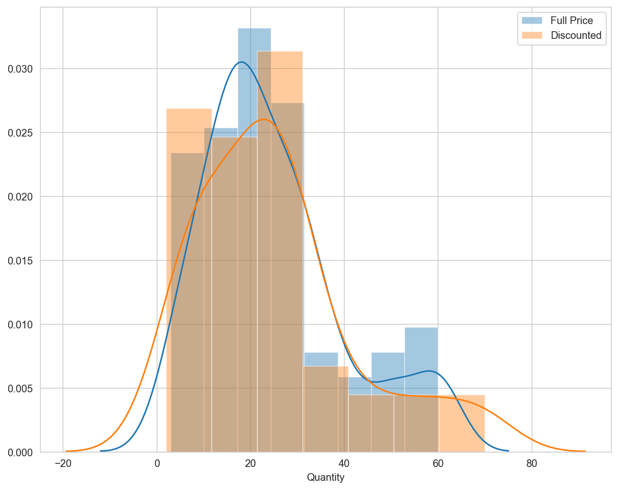
# visually inspect differences in mean and StDev of distributions
sns.set_style("whitegrid")
%config InlineBackend.figure_format='retina'
%matplotlib inline
fig = plt.figure(figsize=(10,8))
ax = fig.gca()

ax.axvline(fullprice.mean(), color='blue', lw=2, ls='--', label='FP Avg')
ax.axvline(discount.mean(), color='orange', lw=2, ls='--', label='DC Avg')

fdict = {'fontfamily': 'PT Mono','fontsize': 16}

sns.distplot(fullprice, ax=ax, hist=True, kde=True, color='blue')
sns.distplot(discount, ax=ax, hist=True, kde=True, color='orange')
ax.legend(['Full Price', 'Discount'])
ax.set_title("Distribution of Full Price vs Discount Order Quantity", fontdict=fdict)

Text(0.5, 1.0, 'Distribution of Full Price vs Discount Order Quantity')

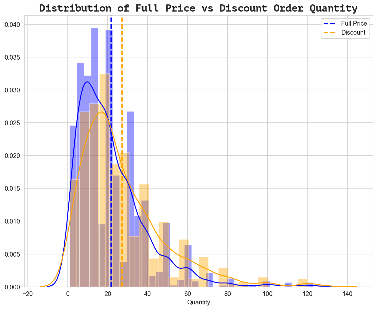
fig = plt.figure(figsize=(10,8))
ax = fig.gca()
ax = sns.barplot(x='Discount', y='Quantity', data=df_orderDetail)
ax.set_title('Discount Levels and Order Qty', fontdict={'family': 'PT Mono', 'size':16})

Text(0.5, 1.0, 'Discount Levels and Order Qty')

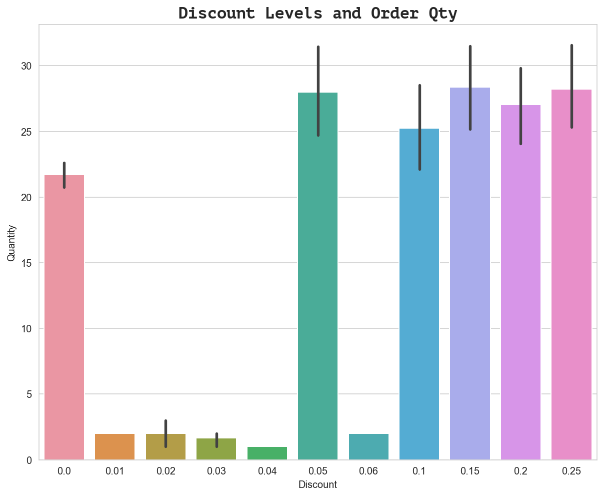
We can already see that there is a clear relationship between order quantity and specific discount levels before running any statistical tests. However, what is more interesting to note from the visualization above is that the discount levels that DO have an effect appear to be very similar as far as the mean order quantity. The indication is that discount amount produces diminishing returns (offering a discount higher than 5% - the minimum effective amount - does not actually produce higher order quantity which means we are losing revenue we would have otherwise captured).

Assumption Tests

Select the appropriate t-test based on tests for the assumptions of normality and homogeneity of variance.

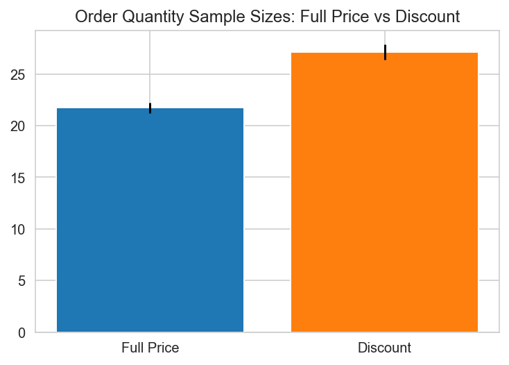
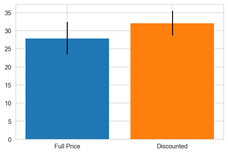
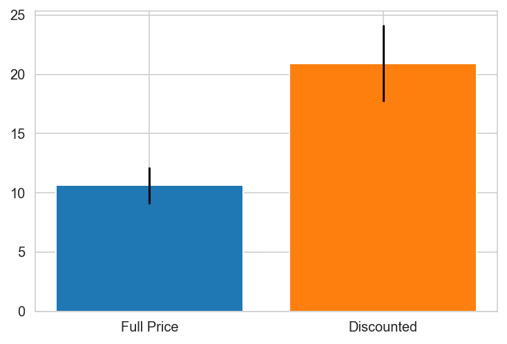
Sample Size

Check if sample sizes allow us to ignore assumptions; if not, test assumption normality.

# visualize sample size comparisons for two groups (normality check)
import scipy.stats as stat
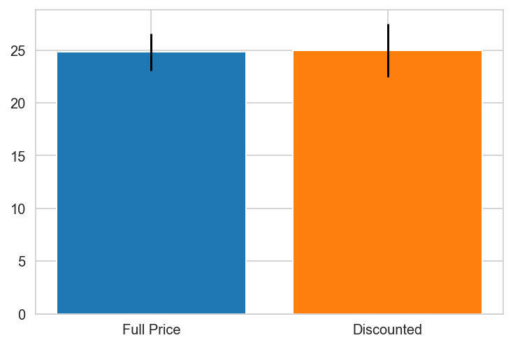
plt.bar(x='Full Price', height=fullprice.mean(), yerr=stat.sem(fullprice))
plt.bar(x='Discount', height=discount.mean(), yerr=stat.sem(discount))
plt.title("Order Quantity Sample Sizes: Full Price vs Discount")

Text(0.5, 1.0, 'Order Quantity Sample Sizes: Full Price vs Discount')

Normality Test

Check assumptions of normality and homogeneity of variance

# Test for normality - D'Agostino-Pearson's normality test: scipy.stats.normaltest
stat.normaltest(fullprice), stat.normaltest(discount)

(NormaltestResult(statistic=544.5770045551502, pvalue=5.579637380545965e-119),
 NormaltestResult(statistic=261.528012299789, pvalue=1.6214878452829618e-57))

Failed normality test (p-values < 0.05). Run non-parametric test:

# Run non-parametric test (since normality test failed)
stat.mannwhitneyu(fullprice, discount)

MannwhitneyuResult(statistic=461541.0, pvalue=6.629381826999866e-11)

Statistical Test

Perform chosen statistical test.

# run tukey test for OQD (Order Quantity Discount) 
data = df_orderDetail['Quantity'].values
labels = df_orderDetail['Discount'].values

import statsmodels.api as sms
model = sms.stats.multicomp.pairwise_tukeyhsd(data,labels)

# save OQD tukey test model results into dataframe (OQD: order quantity discount)
tukey_OQD = pd.DataFrame(data=model._results_table[1:], columns=model._results_table[0])
tukey_OQD

	group1	group2	meandiff	p-adj	lower	upper	reject
0	0.0	0.01	-19.7153	0.9	-80.3306	40.9001	False
1	0.0	0.02	-19.7153	0.9	-62.593	23.1625	False
2	0.0	0.03	-20.0486	0.725	-55.0714	14.9742	False
3	0.0	0.04	-20.7153	0.9	-81.3306	39.9001	False
4	0.0	0.05	6.2955	0.0011	1.5381	11.053	True
5	0.0	0.06	-19.7153	0.9	-80.3306	40.9001	False
6	0.0	0.1	3.5217	0.4269	-1.3783	8.4217	False
7	0.0	0.15	6.6669	0.0014	1.551	11.7828	True
8	0.0	0.2	5.3096	0.0303	0.2508	10.3684	True
9	0.0	0.25	6.525	0.0023	1.3647	11.6852	True
10	0.01	0.02	0.0	0.9	-74.2101	74.2101	False
11	0.01	0.03	-0.3333	0.9	-70.2993	69.6326	False
12	0.01	0.04	-1.0	0.9	-86.6905	84.6905	False
13	0.01	0.05	26.0108	0.9	-34.745	86.7667	False
14	0.01	0.06	0.0	0.9	-85.6905	85.6905	False
15	0.01	0.1	23.237	0.9	-37.5302	84.0042	False
16	0.01	0.15	26.3822	0.9	-34.4028	87.1671	False
17	0.01	0.2	25.0248	0.9	-35.7554	85.805	False
18	0.01	0.25	26.2403	0.9	-34.5485	87.029	False
19	0.02	0.03	-0.3333	0.9	-55.6463	54.9796	False
20	0.02	0.04	-1.0	0.9	-75.2101	73.2101	False
21	0.02	0.05	26.0108	0.6622	-17.0654	69.087	False
22	0.02	0.06	0.0	0.9	-74.2101	74.2101	False
23	0.02	0.1	23.237	0.7914	-19.8552	66.3292	False
24	0.02	0.15	26.3822	0.6461	-16.7351	69.4994	False
25	0.02	0.2	25.0248	0.7089	-18.0857	68.1354	False
26	0.02	0.25	26.2403	0.6528	-16.8823	69.3628	False
27	0.03	0.04	-0.6667	0.9	-70.6326	69.2993	False
28	0.03	0.05	26.3441	0.3639	-8.9214	61.6096	False
29	0.03	0.06	0.3333	0.9	-69.6326	70.2993	False
30	0.03	0.1	23.5703	0.5338	-11.7147	58.8553	False
31	0.03	0.15	26.7155	0.3436	-8.6001	62.0311	False
32	0.03	0.2	25.3582	0.428	-9.9492	60.6656	False
33	0.03	0.25	26.5736	0.3525	-8.7485	61.8957	False
34	0.04	0.05	27.0108	0.9	-33.745	87.7667	False
35	0.04	0.06	1.0	0.9	-84.6905	86.6905	False
36	0.04	0.1	24.237	0.9	-36.5302	85.0042	False
37	0.04	0.15	27.3822	0.9	-33.4028	88.1671	False
38	0.04	0.2	26.0248	0.9	-34.7554	86.805	False
39	0.04	0.25	27.2403	0.9	-33.5485	88.029	False
40	0.05	0.06	-26.0108	0.9	-86.7667	34.745	False
41	0.05	0.1	-2.7738	0.9	-9.1822	3.6346	False
42	0.05	0.15	0.3714	0.9	-6.2036	6.9463	False
43	0.05	0.2	-0.986	0.9	-7.5166	5.5447	False
44	0.05	0.25	0.2294	0.9	-6.3801	6.839	False
45	0.06	0.1	23.237	0.9	-37.5302	84.0042	False
46	0.06	0.15	26.3822	0.9	-34.4028	87.1671	False
47	0.06	0.2	25.0248	0.9	-35.7554	85.805	False
48	0.06	0.25	26.2403	0.9	-34.5485	87.029	False
49	0.1	0.15	3.1452	0.9	-3.5337	9.824	False
50	0.1	0.2	1.7879	0.9	-4.8474	8.4231	False
51	0.1	0.25	3.0033	0.9	-3.7096	9.7161	False
52	0.15	0.2	-1.3573	0.9	-8.1536	5.4389	False
53	0.15	0.25	-0.1419	0.9	-7.014	6.7302	False
54	0.2	0.25	1.2154	0.9	-5.6143	8.0451	False

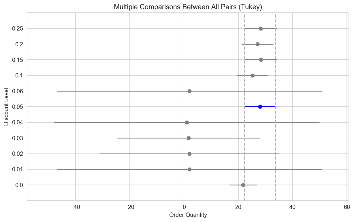
# Plot a universal confidence interval of each group mean comparing significant differences in group means. 
# Significant differences at the alpha=0.05 level can be identified by intervals that do not overlap 

oq_data = df_orderDetail['Quantity'].values
discount_labels = df_orderDetail['Discount'].values

from statsmodels.stats.multicomp import MultiComparison
oqd = MultiComparison(oq_data, discount_labels)
results = oqd.tukeyhsd()
results.plot_simultaneous(comparison_name=0.05, xlabel='Order Quantity', ylabel='Discount Level');

Effect Size

Calculate effect size using Cohen’s D as well as any post-hoc tests.

#### Cohen's d
def Cohen_d(group1, group2):
    # Compute Cohen's d.
    # group1: Series or NumPy array
    # group2: Series or NumPy array
    # returns a floating point number 
    diff = group1.mean() - group2.mean()

    n1, n2 = len(group1), len(group2)
    var1 = group1.var()
    var2 = group2.var()

    # Calculate the pooled threshold as shown earlier
    pooled_var = (n1 * var1 + n2 * var2) / (n1 + n2)
    
    # Calculate Cohen's d statistic
    d = diff / np.sqrt(pooled_var)
    
    return d

Cohen_d(discount, fullprice)

0.2862724481729282

Post-hoc Tests

The mean quantity per order is similar for each of the discount levels that we identified as significant. The obvious conclusion to draw from this is that offering a discount higher than 5% does not increase the order quantities; higher discounts only produce higher loss in revenue.

# Extract revenue lost per discounted order where discount had no effect on order quantity
cur.execute("""SELECT Discount, 
                SUM(UnitPrice * Quantity) as 'revLoss',
                COUNT(OrderId) as 'NumOrders'
                FROM orderDetail  
                GROUP BY Discount
                HAVING Discount != 0 AND Discount != 0.05
                ORDER BY revLoss DESC;""")
df = pd.DataFrame(cur.fetchall())
df. columns = [i[0] for i in cur.description]
print(len(df))
df.head()

	Discount	revLoss	NumOrders
0	0.25	131918.09	154
1	0.20	111476.38	161
2	0.15	102948.44	157
3	0.10	101665.71	173
4	0.03	124.65	3

print("Total Revenue Forfeited $", df.revLoss.sum())
print("Number of Orders Affected ", df.NumOrders.sum())
print("Avg Forfeited Per Order $", df.revLoss.sum()/df.NumOrders.sum())

Total Revenue Forfeited $ 448373.27
Number of Orders Affected  653
Avg Forfeited Per Order $ 686.6359418070444

Analyze Results

Where alpha = 0.05, the null hypothesis is rejected. Discount amount has a statistically significant effect on the quantity in an order where the discount level is equal to 5%, 15%, 20% or 25%.

H2: Country–Discount

Do individual countries show a statistically significant preference for discount?

If so, which countries and to what extent?

Hypotheses

$H_0$: Countries purchase equal quantities of discounted vs non-discounted products.
$H_A$: Countries purchase different quantities of discounted vs non-discounted products.

EDA

Select the proper dataset for analysis, perform EDA, and generate data groups for testing.

Select

df_order = get_table(cur, "'Order'")
display(df_order.head())
display(df_orderDetail.head())

	OrderId	CustomerId	EmployeeId	OrderDate	RequiredDate	ShippedDate	ShipVia	Freight	ShipName	ShipAddress	ShipCity	ShipRegion	ShipPostalCode	ShipCountry
0	10248	VINET	5	2012-07-04	2012-08-01	2012-07-16	3	32.38	Vins et alcools Chevalier	59 rue de l'Abbaye	Reims	Western Europe	51100	France
1	10249	TOMSP	6	2012-07-05	2012-08-16	2012-07-10	1	11.61	Toms Spezialitäten	Luisenstr. 48	Münster	Western Europe	44087	Germany
2	10250	HANAR	4	2012-07-08	2012-08-05	2012-07-12	2	65.83	Hanari Carnes	Rua do Paço, 67	Rio de Janeiro	South America	05454-876	Brazil
3	10251	VICTE	3	2012-07-08	2012-08-05	2012-07-15	1	41.34	Victuailles en stock	2, rue du Commerce	Lyon	Western Europe	69004	France
4	10252	SUPRD	4	2012-07-09	2012-08-06	2012-07-11	2	51.30	Suprêmes délices	Boulevard Tirou, 255	Charleroi	Western Europe	B-6000	Belgium

	Id	OrderId	ProductId	UnitPrice	Quantity
0	10248/11	10248	11	14.0	12
1	10248/42	10248	42	9.8	10
2	10248/72	10248	72	34.8	5
3	10249/14	10249	14	18.6	9
4	10249/51	10249	51	42.4	40

# Rename 'Id' to 'OrderId' for joining tables with matching primary key name
df_order.rename({'Id':'OrderId'}, axis=1, inplace=True)
display(df_order.head())

	OrderId	CustomerId	EmployeeId	OrderDate	RequiredDate	ShippedDate	ShipVia	Freight	ShipName	ShipAddress	ShipCity	ShipRegion	ShipPostalCode	ShipCountry
0	10248	VINET	5	2012-07-04	2012-08-01	2012-07-16	3	32.38	Vins et alcools Chevalier	59 rue de l'Abbaye	Reims	Western Europe	51100	France
1	10249	TOMSP	6	2012-07-05	2012-08-16	2012-07-10	1	11.61	Toms Spezialitäten	Luisenstr. 48	Münster	Western Europe	44087	Germany
2	10250	HANAR	4	2012-07-08	2012-08-05	2012-07-12	2	65.83	Hanari Carnes	Rua do Paço, 67	Rio de Janeiro	South America	05454-876	Brazil
3	10251	VICTE	3	2012-07-08	2012-08-05	2012-07-15	1	41.34	Victuailles en stock	2, rue du Commerce	Lyon	Western Europe	69004	France
4	10252	SUPRD	4	2012-07-09	2012-08-06	2012-07-11	2	51.30	Suprêmes délices	Boulevard Tirou, 255	Charleroi	Western Europe	B-6000	Belgium

df_order.set_index('OrderId',inplace=True)
display(df_order.head())

	CustomerId	EmployeeId	OrderDate	RequiredDate	ShippedDate	ShipVia	Freight	ShipName	ShipAddress	ShipCity	ShipRegion	ShipPostalCode	ShipCountry
OrderId
10248	VINET	5	2012-07-04	2012-08-01	2012-07-16	3	32.38	Vins et alcools Chevalier	59 rue de l'Abbaye	Reims	Western Europe	51100	France
10249	TOMSP	6	2012-07-05	2012-08-16	2012-07-10	1	11.61	Toms Spezialitäten	Luisenstr. 48	Münster	Western Europe	44087	Germany
10250	HANAR	4	2012-07-08	2012-08-05	2012-07-12	2	65.83	Hanari Carnes	Rua do Paço, 67	Rio de Janeiro	South America	05454-876	Brazil
10251	VICTE	3	2012-07-08	2012-08-05	2012-07-15	1	41.34	Victuailles en stock	2, rue du Commerce	Lyon	Western Europe	69004	France
10252	SUPRD	4	2012-07-09	2012-08-06	2012-07-11	2	51.30	Suprêmes délices	Boulevard Tirou, 255	Charleroi	Western Europe	B-6000	Belgium

df_country = df_orderDetail.merge(df_order, on='OrderId', copy=True)

Explore

fs.ft.alphasentaurii.hot_stats(df_country, 'ShipCountry')

-------->
HOT!STATS
<--------

SHIPCOUNTRY
Data Type: object

min    Argentina
max    Venezuela
Name: ShipCountry, dtype: object 

à-la-Mode: 
0    USA
dtype: object


No Nulls Found!

Non-Null Value Counts:
USA            352
Germany        328
Brazil         203
France         184
UK             135
Austria        125
Venezuela      118
Sweden          97
Canada          75
Mexico          72
Belgium         56
Ireland         55
Spain           54
Finland         54
Italy           53
Switzerland     52
Denmark         46
Argentina       34
Portugal        30
Poland          16
Norway          16
Name: ShipCountry, dtype: int64

# Unique Values: 21

Group

countries = df_country.groupby('ShipCountry').groups
countries.keys()

dict_keys(['Argentina', 'Austria', 'Belgium', 'Brazil', 'Canada', 'Denmark', 'Finland', 'France', 'Germany', 'Ireland', 'Italy', 'Mexico', 'Norway', 'Poland', 'Portugal', 'Spain', 'Sweden', 'Switzerland', 'UK', 'USA', 'Venezuela'])

df_countries = df_country[['ShipCountry','Quantity','discounted']].copy()
df_countries.ShipCountry.value_counts()

USA            352
Germany        328
Brazil         203
France         184
UK             135
Austria        125
Venezuela      118
Sweden          97
Canada          75
Mexico          72
Belgium         56
Ireland         55
Spain           54
Finland         54
Italy           53
Switzerland     52
Denmark         46
Argentina       34
Portugal        30
Poland          16
Norway          16
Name: ShipCountry, dtype: int64

import researchpy as rp
rp.summary_cont(df_countries.groupby(['discounted']))

	Quantity
	N	Mean	SD	SE	95% Conf.	Interval
discounted
0	1317	21.715262	17.507493	0.482426	20.769706	22.660818
1	838	27.109785	20.771439	0.717537	25.703412	28.516159

Test

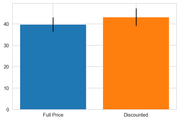
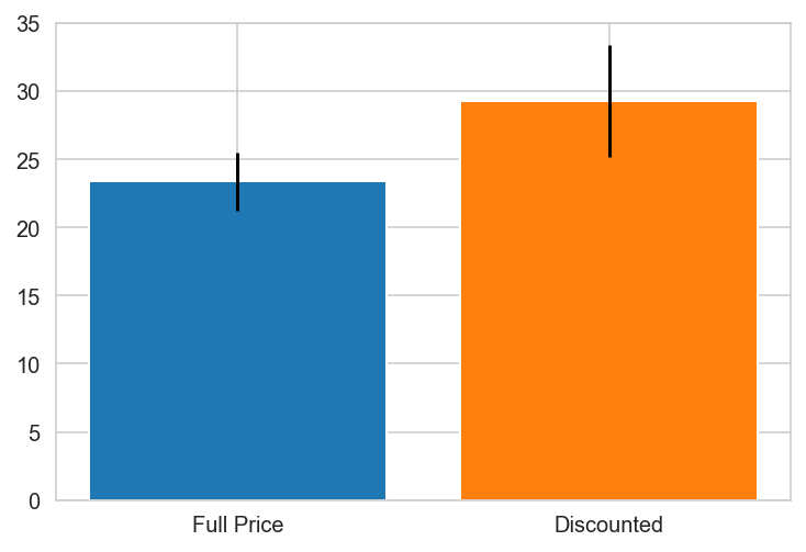
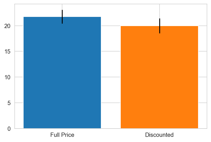
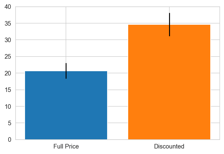
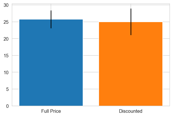
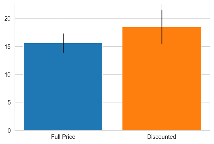
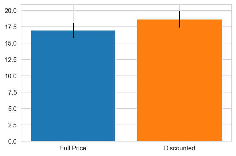
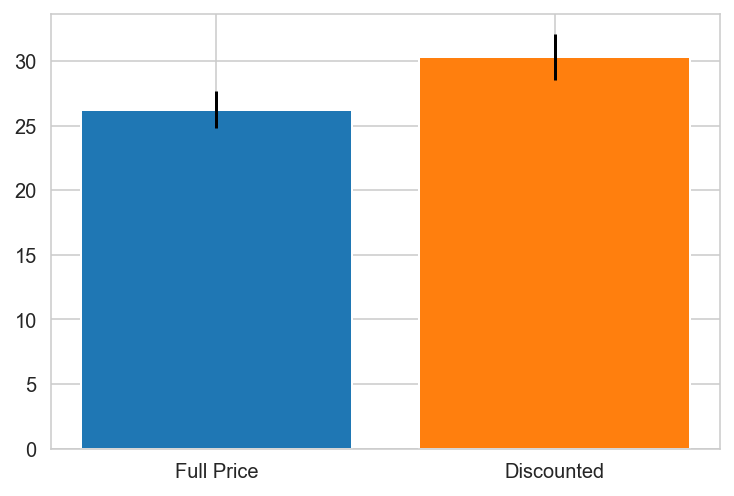
Sample Size

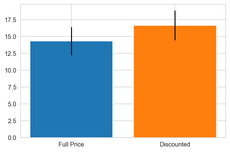
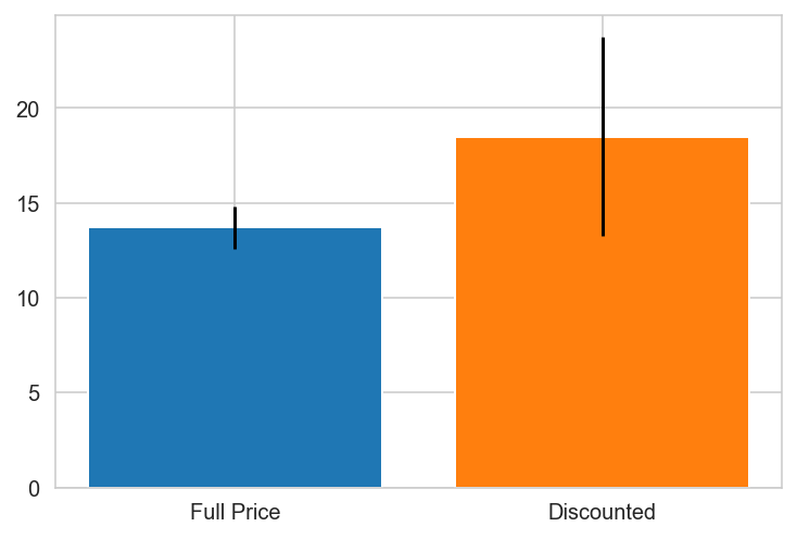
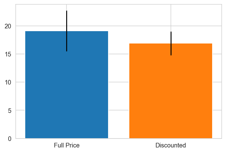
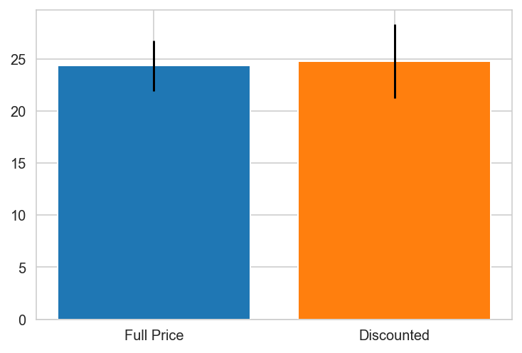
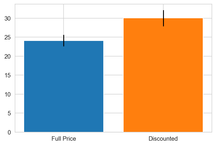
# Check if sample sizes allow us to ignore assumptions;
# visualize sample size comparisons for two groups (normality check)

stat_dict = {}

for k,v in countries.items():
    try:
        grp0 = df_countries.loc[v].groupby('discounted').get_group(0)['Quantity']
        grp1 = df_countries.loc[v].groupby('discounted').get_group(1)['Quantity']
        print(f"{k}")
        
        import scipy.stats as stat

        plt.bar(x='Full Price', height=grp0.mean(), yerr=stat.sem(grp0))
        plt.bar(x='Discounted', height=grp1.mean(), yerr=stat.sem(grp1))
        plt.show()
        
    except:
        pass
        
    try:
        result = stat.ttest_ind(grp0,grp1)
        if result[1] < 0.05:
            stat_dict[k] = result[1]
            print(f"\n{k} PREFERS DISCOUNTS!")
        else:
            continue
    except:
        print(f"{k} does not contain one of the groups.")
stat_dict

Argentina does not contain one of the groups.
Austria

Belgium

Brazil

Canada

Canada PREFERS DISCOUNTS!
Denmark

Finland

France

Germany

Ireland

Italy

Mexico

Norway PREFERS DISCOUNTS!
Portugal

Spain

Spain PREFERS DISCOUNTS!
Sweden

Switzerland

UK

UK PREFERS DISCOUNTS!
USA

USA PREFERS DISCOUNTS!
Venezuela

{'Canada': 0.0010297982736886485,
 'Norway': 0.04480094051665529,
 'Spain': 0.0025087181106716217,
 'UK': 0.00031794803200322925,
 'USA': 0.019868707223971476}

stat_dict

{'Canada': 0.0010297982736886485,
 'Norway': 0.04480094051665529,
 'Spain': 0.0025087181106716217,
 'UK': 0.00031794803200322925,
 'USA': 0.019868707223971476}

Normality Test

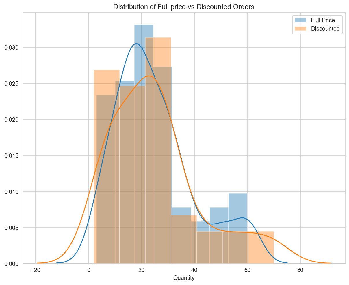
fig = plt.figure(figsize=(10,8))
ax = fig.gca(title="Distribution of Full price vs Discounted Orders")

sns.distplot(grp0)
sns.distplot(grp1)
ax.legend(['Full Price','Discounted'])

<matplotlib.legend.Legend at 0x1a25ab2978>

# Test for normality - D'Agostino-Pearson's normality test: scipy.stats.normaltest
stat.normaltest(grp0), stat.normaltest(grp1)

(NormaltestResult(statistic=9.316225653095811, pvalue=0.009484344125890621),
 NormaltestResult(statistic=10.255309993341813, pvalue=0.005930451108115991))

# Run non-parametric test (since normality test failed)
stat.mannwhitneyu(grp0, grp1)

MannwhitneyuResult(statistic=1632.5, pvalue=0.44935140740973323)

Canada, Spain, UK and the USA have pvalues < 0.05 indicating there is a relationship between discount and order quantity and the null hypothesis is rejected for these individual countries.

Statistical Test

import statsmodels.api as sm
from statsmodels.formula.api import ols
model = ols("Quantity~C(discounted)+C(ShipCountry)+C(discounted):C(ShipCountry)", data=df_countries).fit()
anova_table = sm.stats.anova_lm(model, typ=2)

/Users/alphasentaurii/opt/anaconda3/envs/learn-env/lib/python3.6/site-packages/statsmodels/base/model.py:1752: ValueWarning: covariance of constraints does not have full rank. The number of constraints is 20, but rank is 18
  'rank is %d' % (J, J_), ValueWarning)
/Users/alphasentaurii/opt/anaconda3/envs/learn-env/lib/python3.6/site-packages/statsmodels/base/model.py:1752: ValueWarning: covariance of constraints does not have full rank. The number of constraints is 20, but rank is 18
  'rank is %d' % (J, J_), ValueWarning)

# reformat scientific notation of results for easier interpretation
anova_table.style.format("{:.5f}", subset=['PR(>F)'])

	sum_sq	df	F	PR(>F)
C(discounted)	9.78092e-08	1	3.07557e-10	0.99999
C(ShipCountry)	101347	20	15.9341	0.00000
C(discounted):C(ShipCountry)	15584.9	20	2.4503	0.00061
Residual	672930	2116	nan	nan

# calculate ttest_ind p-values and significance for individual countries
print(f"\n Countries with p-values < 0.05 - Null Hypothesis Rejected:")
for k,v in countries.items():
    try:
        grp0 = df_countries.loc[v].groupby('discounted').get_group(0)['Quantity']
        grp1 = df_countries.loc[v].groupby('discounted').get_group(1)['Quantity']
        result = stat.ttest_ind(grp0,grp1)
        if result[1] < 0.05:
            
            print(f"\n\t{k}: {result[1].round(4)}")
        else:
            continue
    except:
        None 

 Countries with p-values < 0.05 - Null Hypothesis Rejected:

	Canada: 0.001

	Spain: 0.0025

	UK: 0.0003

	USA: 0.0199

Although discount does not have a significant effect on countries overall (p = 0.99), there is a statistically significant relationship between order quantities and discount in some of the countries (p=0.0006).

Countries with p-values < 0.05 - Null Hypothesis Rejected:

Canada: 0.001

Spain: 0.0025

UK: 0.0003

USA: 0.0199

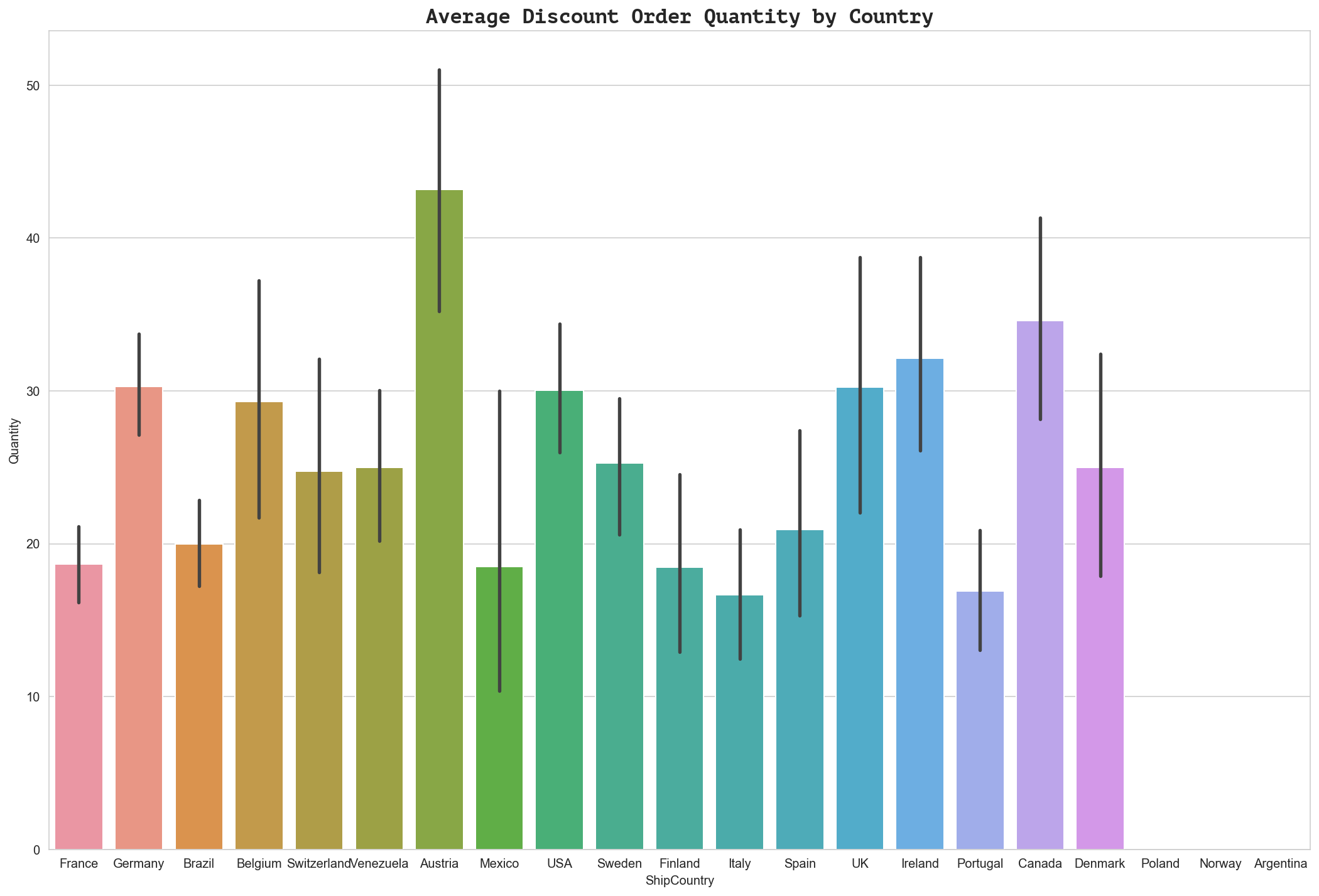
y1 = df_countries.groupby('discounted').get_group(1)['Quantity']

fig = plt.figure(figsize=(18,12))
ax = fig.gca()

ax = sns.barplot(x='ShipCountry', y=y1, data=df_countries)

ax.set_title('Average Discount Order Quantity by Country', fontdict={'family': 'PT Mono', 'size':16})

Text(0.5, 1.0, 'Average Discount Order Quantity by Country')

Effect Size

Effect size testing is unnecessary since the null hypothesis for the main question was not rejected.

Post-hoc Tests

#!pip install pandasql
from pandasql import sqldf
pysqldf = lambda q: sqldf(q, globals())

# Compare number of discount vs fullprice orders by country.
# Create bar plots grouped as discount vs fullprice orders by country
#fig, axes = plt.subplots(nrows=1, ncols=1, figsize=(18,8))

q1 = "SELECT ShipCountry, AVG(Quantity) as OrderQty from df_countries where discounted = 0 group by 1;"
q2 = "SELECT ShipCountry, AVG(Quantity) as OrderQty from df_countries where discounted = 1 group by 1;"

df_fpCount = pysqldf(q1)
df_dcCount = pysqldf(q2)

df_fpCount['Group'] = 'FullPrice'
df_dcCount['Group'] = 'Discount'

df_country_qty = pd.concat([df_fpCount, df_dcCount], axis=0)

display(df_country_qty.describe())

#ax = sns.barplot(x='ShipCountry', y='NumOrders', data=country_df, hue='Group', palette='pastel', orient='v')
#ax.set_title('Number of Fullprice vs Discount Orders by Country', fontdict={'family': 'monospace', 'size':16})

#ax1 = sns.barplot(x='ShipCountry', y='TotalQty', data=country_df, hue='Group', palette='pastel', orient='v')
#ax1.set_title('Total Qty of Fullprice vs Discount Orders by Country', fontdict={'family': 'monospace', 'size':16})

sns.set_style("whitegrid")
fig = plt.figure(figsize=(18,8))
ax = fig.gca(title="Average Order Quantity by Country: Fullprice vs Discount")

sns.barplot(x='ShipCountry', y='OrderQty', ax=ax, data=df_country_qty, hue='Group', 
            palette='pastel', orient='v', ci=68, capsize=.2)

## Set Title,X/Y Labels,fonts,formatting
ax_font = {'family':'monospace','weight':'semibold','size':14}
tick_font = {'size':12,'ha':'center','rotation':45}
t_label = "Average Order Quantity by Country: Fullprice vs Discount Orders"
t_font = {'family': 'PT Mono', 'size':18}

ax.set_ylabel("Order Qty", fontdict=ax_font)
ax.set_xlabel("Country", fontdict=ax_font)
#ax.set_title('Average Order Quantity by Country: Fullprice vs Discount', fontdict={'family': 'PT Mono', 'size':16})
ax.set_title(t_label, fontdict=t_font)

	OrderQty
count	39.000000
mean	22.596281
std	7.620086
min	9.970588
25%	17.458458
50%	21.750000
75%	25.985539
max	43.172414

Text(0.5, 1.0, 'Average Order Quantity by Country: Fullprice vs Discount Orders')

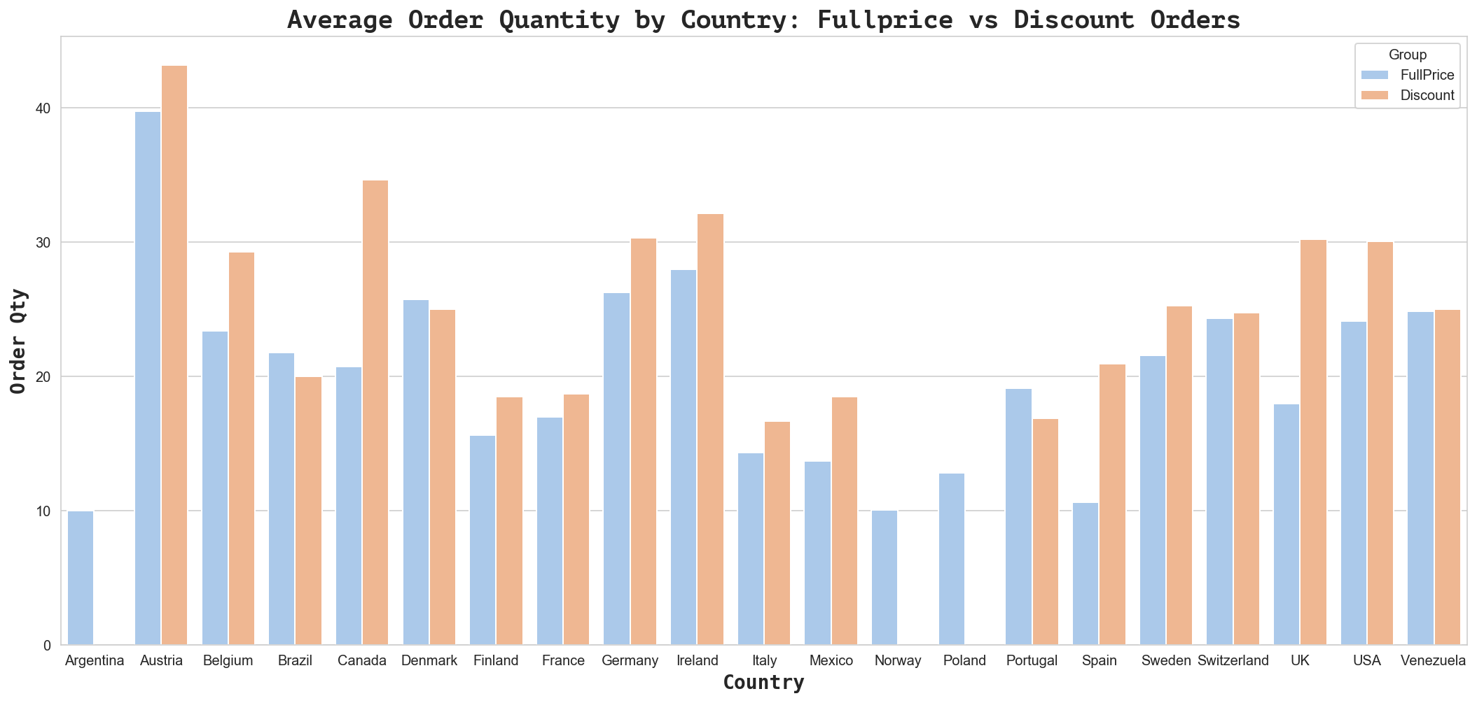
According to the plot above, the actual number of discounted orders is lower than the number of full price orders. Let’s compare the sum of quantities for these orders in each group.

# Compare number of discount vs fullprice orders by country.
# Create bar plots grouped as discount vs fullprice orders by country
#fig, axes = plt.subplots(nrows=1, ncols=1, figsize=(18,8))

q1 = "SELECT ShipCountry, Count(*) as OrderCount from df_countries where discounted = 0 group by 1;"
q2 = "SELECT ShipCountry, Count(*) as OrderCount from df_countries where discounted = 1 group by 1;"

df_fpCount = pysqldf(q1)
df_dcCount = pysqldf(q2)

df_fpCount['Group'] = 'FullPrice'
df_dcCount['Group'] = 'Discount'

df_country_count = pd.concat([df_fpCount, df_dcCount], axis=0)

display(df_country_count.describe())

#ax = sns.barplot(x='ShipCountry', y='NumOrders', data=country_df, hue='Group', palette='pastel', orient='v')
#ax.set_title('Number of Fullprice vs Discount Orders by Country', fontdict={'family': 'monospace', 'size':16})

#ax1 = sns.barplot(x='ShipCountry', y='TotalQty', data=country_df, hue='Group', palette='pastel', orient='v')
#ax1.set_title('Total Qty of Fullprice vs Discount Orders by Country', fontdict={'family': 'monospace', 'size':16})


fig = plt.figure(figsize=(18,8))
ax = fig.gca(title="Mean QPO by Country")

sns.barplot(x='ShipCountry', y='OrderCount', ax=ax, data=df_country_count, hue='Group', palette='Reds_d', 
            orient='v', ci=68, capsize=.2)

## Set Title,X/Y Labels,fonts,formatting
ax_font = {'family':'monospace','weight':'semibold','size':14}
tick_font = {'size':12,'ha':'center','rotation':45}
t_label = "Count of Fullprice vs Discount Orders by Country"
t_font = {'family': 'PT Mono', 'size':18}

ax.set_ylabel("Number of Orders", fontdict=ax_font)
ax.set_xlabel("Country", fontdict=ax_font)
#ax.set_title('Average Order Quantity by Country: Fullprice vs Discount', fontdict={'family': 'PT Mono', 'size':16})
ax.set_title(t_label, fontdict=t_font)

	OrderCount
count	39.000000
mean	55.256410
std	48.722478
min	8.000000
25%	22.000000
50%	39.000000
75%	69.500000
max	210.000000

Text(0.5, 1.0, 'Count of Fullprice vs Discount Orders by Country')

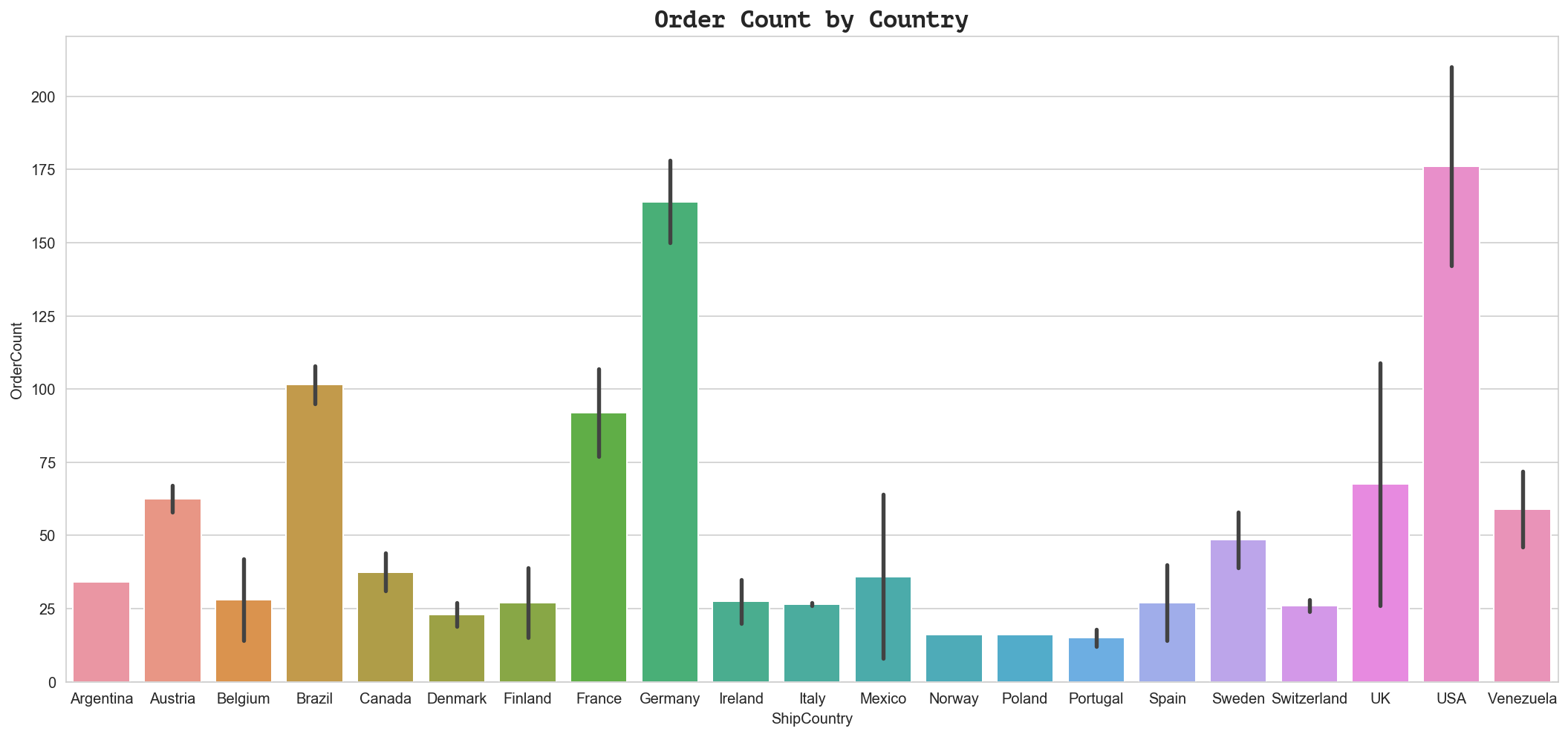
This still doesn’t tell us much about whether or not these countries prefer discounts (tend to order more products) or not - in order to get better insight, we need to look at the average order size (mean quantities per order) for each group.

# Compare number of discount vs fullprice orders by country.
# Create bar plots grouped as discount vs fullprice orders by country
#fig, axes = plt.subplots(nrows=1, ncols=1, figsize=(18,8))

#q1 = "SELECT ShipCountry, Count(*) as NumOrders, SUM(Quantity) as TotalQty, AVG(Quantity) as MeanQPO from df_countries where discounted = 0 group by 1;"
#q2 = "SELECT ShipCountry, Count(*) as NumOrders, SUM(Quantity) as TotalQty, AVG(Quantity) as MeanQPO from df_countries where discounted = 1 group by 1;"

q1 = "SELECT ShipCountry, AVG(Quantity) as MeanQPO from df_countries where discounted = 0 group by 1;"
q2 = "SELECT ShipCountry, AVG(Quantity) as MeanQPO from df_countries where discounted = 1 group by 1;"

fullprice_df = pysqldf(q1)
discount_df = pysqldf(q2)

fullprice_df['Group'] = 'FullPrice'
discount_df['Group'] = 'Discount'

country_df = pd.concat([fullprice_df, discount_df], axis=0)

display(country_df.describe())

#ax = sns.barplot(x='ShipCountry', y='NumOrders', data=country_df, hue='Group', palette='pastel', orient='v')
#ax.set_title('Number of Fullprice vs Discount Orders by Country', fontdict={'family': 'monospace', 'size':16})

#ax1 = sns.barplot(x='ShipCountry', y='TotalQty', data=country_df, hue='Group', palette='pastel', orient='v')
#ax1.set_title('Total Qty of Fullprice vs Discount Orders by Country', fontdict={'family': 'monospace', 'size':16})


fig = plt.figure(figsize=(18,8))
ax = fig.gca(title="Mean QPO by Country")

sns.barplot(x='ShipCountry', y='MeanQPO', ax=ax, data=country_df, hue='Group', palette='Greens_d', 
            orient='v', capsize=.2)

## Set Title,X/Y Labels,fonts,formatting
ax_font = {'family':'monospace','weight':'semibold','size':14}
tick_font = {'size':12,'ha':'center','rotation':45}
t_label = "Average Order Quantity by Country: Fullprice vs Discount"
t_font = {'family': 'PT Mono', 'size':18}

ax.set_ylabel("Avg Qty per Order ", fontdict=ax_font)
ax.set_xlabel("Country", fontdict=ax_font)
#ax.set_title('Average Order Quantity by Country: Fullprice vs Discount', fontdict={'family': 'PT Mono', 'size':16})
ax.set_title(t_label, fontdict=t_font)

	MeanQPO
count	39.000000
mean	22.596281
std	7.620086
min	9.970588
25%	17.458458
50%	21.750000
75%	25.985539
max	43.172414

Text(0.5, 1.0, 'Average Order Quantity by Country: Fullprice vs Discount')

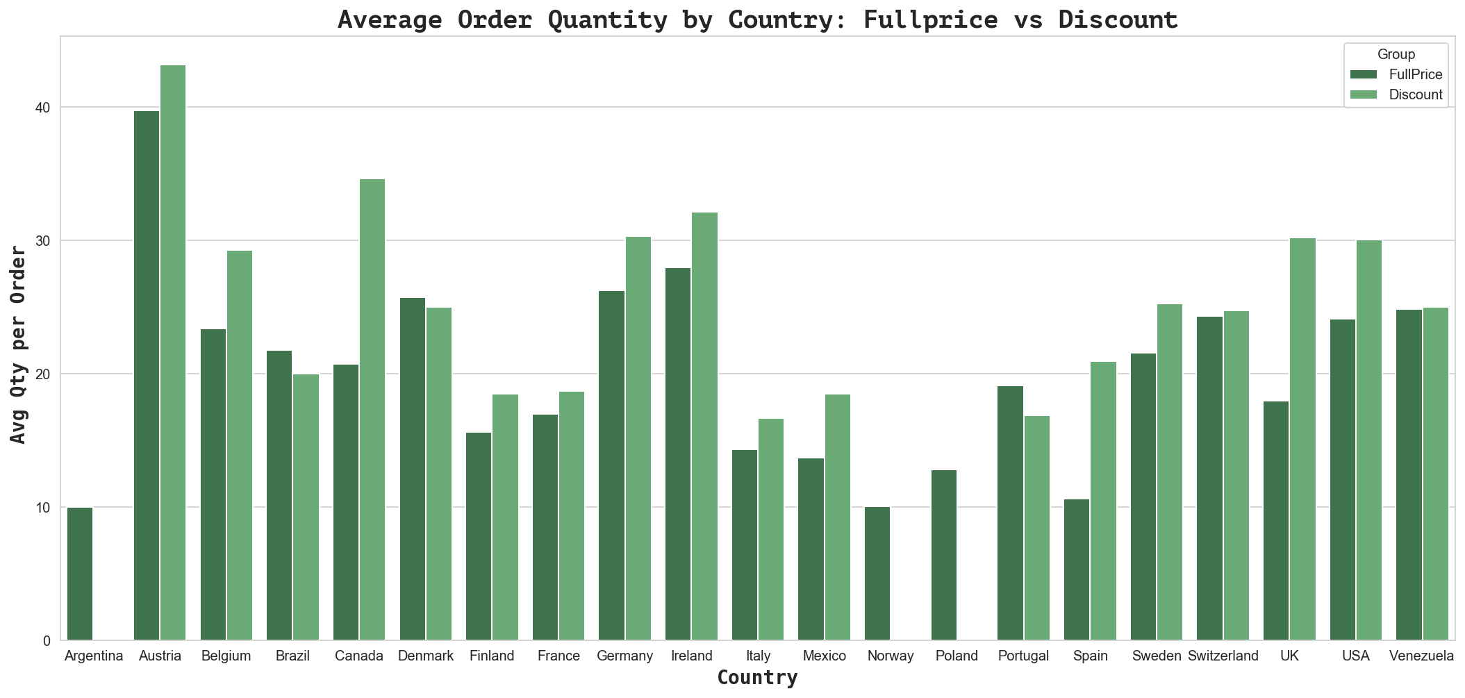
The above plots indicate that when a discount is offered, certain countries order higher quantities of products. Let’s look at the values to determine what percentage more they purchase when an order is discounted.

# add new col for countries where discount has significant effect
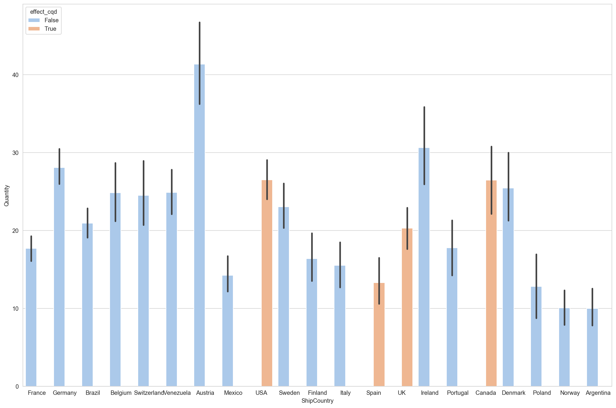
fig = plt.figure(figsize=(18,12))
ax = fig.gca()
df_countries['effect_cqd'] = df_countries['ShipCountry'].isin(['Spain', 'UK', 'USA', 'Canada'])
ax = sns.barplot(x='ShipCountry', y='Quantity', hue='effect_cqd', palette='pastel', data=df_countries)

q1 = "SELECT ShipCountry, Count(*) as OrderCount from df_countries where discounted = 0 group by 1;"
q2 = "SELECT ShipCountry, Count(*) as OrderCount from df_countries where discounted = 1 group by 1;"

df_fpCount = pysqldf(q1)
df_dcCount = pysqldf(q2)

df_fpCount['Group'] = 'FullPrice'
df_dcCount['Group'] = 'Discount'

df_countryCount = pd.concat([df_fpCount, df_dcCount])

fig = plt.figure(figsize=(18,8))
ax = fig.gca(title="Average Order Quantity by Country")

ax = sns.barplot(x='ShipCountry', y='OrderCount', data=df_countryCount)
ax.set_title('Order Count by Country', fontdict={'family': 'PT Mono', 'size':16})

Text(0.5, 1.0, 'Order Count by Country')

Results

For certain individual countries (Spain, Canada, UK, USA), the null hypothesis is rejected with 95% certainty (alpha=0.05)

H3: Region & Revenue

Does average revenue per order vary between different customer regions?

If so, how do the regions rank in terms of average revenue per order?

Additional questions to explore: Does geographic distance between distributor and shipcountry have an effect on order quantity? Does shipping cost have an effect on order quantity?

Hypotheses

$H_0$ the average revenue per order is the same between different customer regions.

$H_1$ Alternate hypothesis: the average revenue per order is different (higher or lower) across different customer regions.

The alpha level (i.e. the probability of rejecting the null hypothesis when it is true) is = 0.05.

EDA

Select the proper dataset for analysis, generate data groups for testing, perform EDA.

Select

# Extract revenue per product per order
cur.execute("""SELECT c.Region, od.OrderId, od.Quantity, od.UnitPrice, od.Discount
FROM Customer c
JOIN 'Order' o ON c.Id = o.CustomerId
JOIN OrderDetail od USING(OrderId);""")
df = pd.DataFrame(cur.fetchall())
df. columns = [i[0] for i in cur.description]
print(len(df))
df.head()

	Region	OrderId	Quantity	UnitPrice
0	Western Europe	10248	12	14.0
1	Western Europe	10248	10	9.8
2	Western Europe	10248	5	34.8
3	Western Europe	10249	9	18.6
4	Western Europe	10249	40	42.4

# Get total revenue per order

df['Revenue'] = df.Quantity * df.UnitPrice * (1-df.Discount)

# Drop unnecessary columns
df.drop(['Quantity', 'UnitPrice', 'Discount'], axis=1, inplace=True)

Group

# Group data by order and get average revenue per order for each region
df_region = df.groupby(['Region', 'OrderId'])['Revenue'].mean().reset_index()
# drop Order Id (no longer necessary)
df_region.drop('OrderId', axis=1, inplace=True)
# check changes
df_region.head()

	Region	Revenue
0	British Isles	239.70
1	British Isles	661.25
2	British Isles	352.40
3	British Isles	258.40
4	British Isles	120.20

# Explore sample sizes before testing: n > 30 to pass assumptions
df_region.groupby('Region').count()

	Revenue
Region
British Isles	75
Central America	21
Eastern Europe	7
North America	152
Northern Europe	55
Scandinavia	28
South America	127
Southern Europe	64
Western Europe	272

Some of the sample sizes are too small to ignore assumptions of normality. We can combine some regions to meet the required threshold of n > 30.

# Group sub-regions together to create sample sizes adequately large for ANOVA testing  (min 30)

# Group Scandinavia, Northern and Eastern Europe
df_region.loc[(df_region.Region == 'Scandinavia') | (df_region.Region == 'Eastern Europe') | (df_region.Region == 'Northern Europe'), 'Region'] = 'North Europe'

# Group South and Central America
df_region.loc[(df_region.Region == 'South America') | (df_region.Region == 'Central America'), 'Region'] = 'South Americas'

# Review sizes of new groups
df_region.groupby('Region').count()

	Revenue
Region
British Isles	75
North America	152
North Europe	90
South Americas	148
Southern Europe	64
Western Europe	272

Explore

fig = plt.figure(figsize=(10,8))
ax = fig.gca()

sns.distplot(grp0)
sns.distplot(grp1)
ax.legend(['Full Price','Discounted'])

# Plot number of orders, total revenue, and average revenue per order by region
fig, (ax1, ax2, ax3) = plt.subplots(3, 1, figsize=(8,8))
# Number of orders
df_region.groupby(['Region'])['Revenue'].count().plot(kind='barh', ax=ax1, color='b')

# Total Revenue
df_region.groupby(['Region'])['Revenue'].sum().plot(kind='barh', ax=ax2, color='r')

# Average Revenue
df_region.groupby(['Region'])['Revenue'].mean().plot(kind='barh', ax=ax3, color='g')

# Label plots and axes
ax1.set_title('Total Orders')
ax1.set_ylabel('')
ax2.set_title('Total Revenue in US$')
ax2.set_ylabel('')
ax3.set_title('Average Revenue per Order US$')
ax3.set_ylabel('')

fig.subplots_adjust(hspace=0.4);

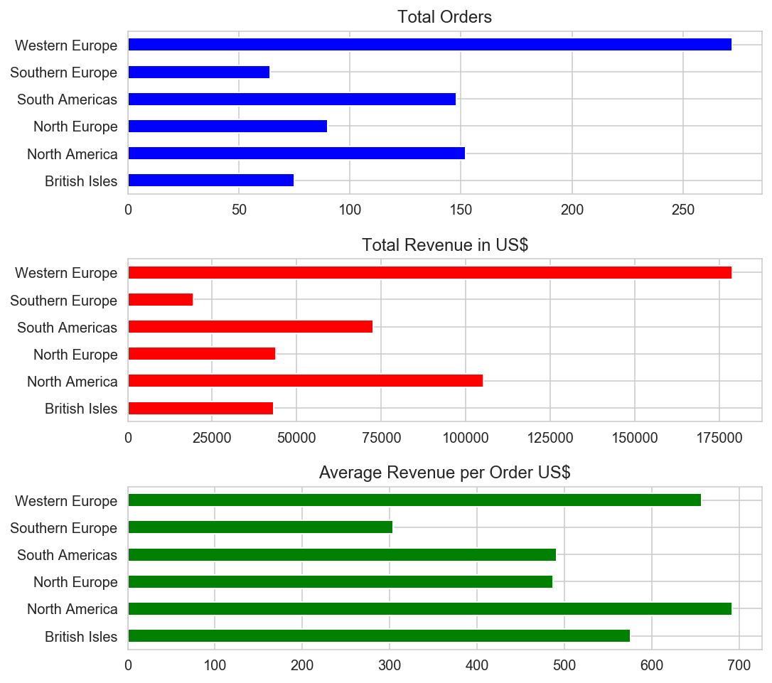
The graphs show that Western Europe is the region with the greatest number of orders, and also has the greatest total revenue. However, North America has the most expensive order on average (followed by Western Europe). Southern and Eastern Europe has the lowest number of orders, lowest total revenue, and cheapest order on average. The third graph lent support to the alternate hypothesis that there are significant differences in average order revenue between regions.

Test

Sample Size

Check if sample sizes allow us to ignore assumptions of normality

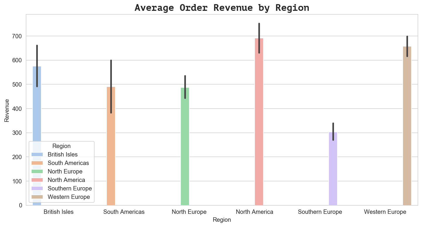
# visualize sample size comparisons, check normality (pvals)
fig = plt.figure(figsize=(12,6))
ax = fig.gca()

ax = sns.barplot(x='Region', y='Revenue', data=df_region, ci=68, palette="pastel", hue='Region')
ax.set_title('Average Order Revenue by Region', fontdict={'family': 'PT Mono', 'size':16})

Text(0.5, 1.0, 'Average Order Revenue by Region')

Normality

Statistical

import statsmodels.api as sm
from statsmodels.formula.api import ols
model = ols("Revenue~C(Region)+Revenue:C(Region)", data=df_region).fit()
anova_table = sm.stats.anova_lm(model, typ=2)
# reformat scientific notation of results for easier interpretation
anova_table.style.format("{:.5f}", subset=['PR(>F)'])

	sum_sq	df	F	PR(>F)
C(Region)	1.03486e+07	5	3.98262e+30	0.00000
Revenue:C(Region)	5.34162e+08	6	1.71309e+32	0.00000
Residual	4.10034e-22	789	nan	nan

# run tukey test for OQD (Order Quantity Discount) 
data = df_region['Revenue'].values
labels = df_region['Region'].values

import statsmodels.api as sms
model = sms.stats.multicomp.pairwise_tukeyhsd(data,labels)

# save OQD tukey test model results into dataframe (OQD: order quantity discount)
tukey_OQD = pd.DataFrame(data=model._results_table[1:], columns=model._results_table[0])
tukey_OQD

	group1	group2	meandiff	p-adj	lower	upper	reject
0	British Isles	North America	116.4615	0.9	-213.9625	446.8854	False
1	British Isles	North Europe	-88.1693	0.9	-454.2704	277.9318	False
2	British Isles	South Americas	-84.2501	0.9	-416.146	247.6458	False
3	British Isles	Southern Europe	-271.7815	0.3745	-670.2535	126.6904	False
4	British Isles	Western Europe	81.6889	0.9	-223.7052	387.083	False
5	North America	North Europe	-204.6308	0.4191	-516.0716	106.8101	False
6	North America	South Americas	-200.7115	0.2778	-471.1191	69.6961	False
7	North America	Southern Europe	-388.243	0.0191	-737.1631	-39.3228	True
8	North America	Western Europe	-34.7725	0.9	-271.9032	202.3581	False
9	North Europe	South Americas	3.9193	0.9	-309.0829	316.9214	False
10	North Europe	Southern Europe	-183.6122	0.7177	-566.4899	199.2655	False
11	North Europe	Western Europe	169.8582	0.5251	-114.889	454.6055	False
12	South Americas	Southern Europe	-187.5315	0.6259	-537.8459	162.783	False
13	South Americas	Western Europe	165.939	0.3541	-73.2385	405.1164	False
14	Southern Europe	Western Europe	353.4704	0.0242	28.1539	678.787	True

North America and Southern Europe: pval = 0.01, mean diff: -388.24

Southern Europe and Western Europe: pval = 0.02, mean diff: 353.4704

Effect Size

Cohen’s D

northamerica = df_region.loc[df_region['Region'] == 'North America']
southerneurope = df_region.loc[df_region['Region'] == 'Southern Europe']
westerneurope = df_region.loc[df_region['Region'] == 'Western Europe']

na_se = Cohen_d(northamerica.Revenue, southerneurope.Revenue)
se_we = Cohen_d(southerneurope.Revenue, westerneurope.Revenue)

print(na_se, se_we)

0.5891669383438923 -0.5462384714677272

Post-Hoc Tests

# log-transforming revenue per order
logRegion_df = df_region.copy()
logRegion_df['Revenue'] = np.log(df_region['Revenue'])

# Plotting the distributions for the log-transformed data
sns.set_style("whitegrid")

fig = plt.figure(figsize=(12,8))
ax = fig.gca(title="Distribution of Revenue Per Order by Region")

for region in set(logRegion_df.Region):
    region_group = logRegion_df.loc[logRegion_df['Region'] == region]
    sns.distplot(region_group['Revenue'], hist_kws=dict(alpha=0.5), label=region)
    ax.legend()
    ax.set_label('Revenue per Order (log-transformed)')

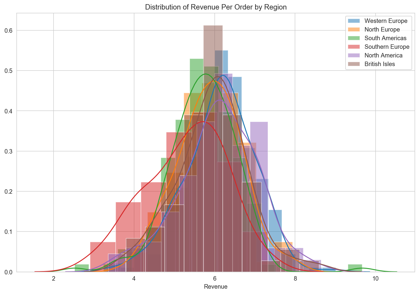
# The data is more normally distributed, and variances from the mean were more similar. 
# run an ANOVA test:

# Fitting a model of revenue per order on Region categories - ANOVA table
lm = ols('Revenue ~ C(Region)', logRegion_df).fit()
sm.stats.anova_lm(lm, typ=2)

	sum_sq	df	F	PR(>F)
C(Region)	48.004167	5.0	12.076998	2.713885e-11
Residual	631.999979	795.0	NaN	NaN

Results

At an alpha level of 0.05 significance, revenue does vary between regions and therefore the null hypothesis is rejected.

The ANOVA table above revealed that the p-value is lower than the alpha value of 0.05. Therefore I was able to reject the null hypothesis and accept the alternate hypothesis. There are statistically significant differences in average order value between different regions, i.e. customers from different parts of the world spend different amounts of money on their orders, on average. Conclusions Business insights: There are statistically significant differences in the average revenue per order from customers from different regions. Western European customers place the most orders, and are the single biggest contributors to Northwind’s bottom line. However, although North American customers have placed roughly half as many orders as those from Western Europe, they spend more per order, on average. The difference between the region with the most expensive orders on average (North America, $1,945.93) and the region with the least expensive orders (Southern and Eastern Europe, $686.73) is $1,259.20, or 2.8 times more for orders from North America. Southern and Eastern Europe has the smallest number of orders, the lowest total revenue, and the lowest average revenue per order. North American customers have placed a similar number of orders to those from South and Central America, but their average expenditure per order is 1.8 times higher. Potential business actions and directions for future work: If Northwind was looking to focus on more profitable customers, a potential action would be to stop serving customers in Southern and Eastern Europe, and to focus more on customers in Western Europe and North America. However, further analysis would be needed to confirm these findings. For example, it might be the case that some more expensive products are only available in certain regions.

H4: Season+Quantity:ProductCategory

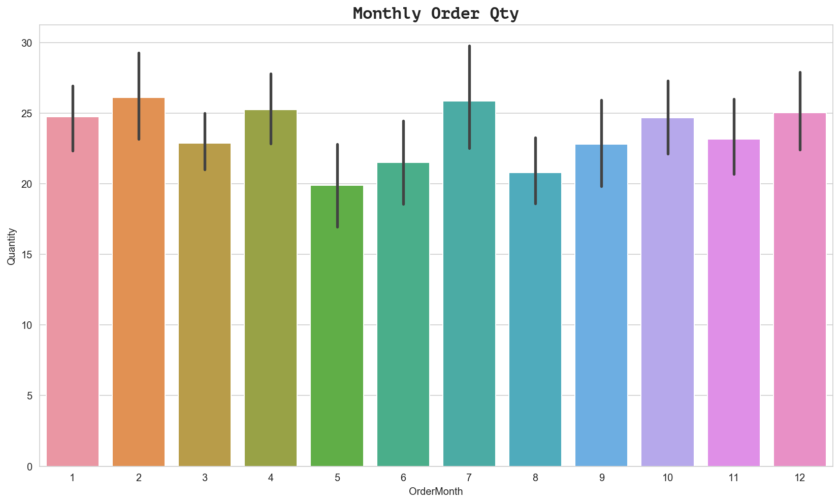
1: Does time of year (month) have an effect on order quantity overall?

2: Does time of year (month) have an effect on order quantity of specific product categories?

3: Does time of year (month) have an effect on order quantity by region?

Hypotheses

$𝐻_1$ : Time of year has a statistically significant effect on average quantity per order.
$𝐻_0$ : Time of year has no relationship with average quantity per order.

EDA

Select proper dataset for analysis: orderDetail, order
Generate data groups for testing: number of orders per month, order quantity per month
Explore data (sample sizes, distribution/density)

Select

df_months = df_orderDetail.merge(df_order, on='OrderId', copy=True)
df_months.head()

	Id	OrderId	ProductId	UnitPrice	Quantity	CustomerId	EmployeeId	OrderDate	RequiredDate	ShippedDate	ShipVia	Freight	ShipName	ShipAddress	ShipCity	ShipRegion	ShipPostalCode	ShipCountry
0	10248/11	10248	11	14.0	12	VINET	5	2012-07-04	2012-08-01	2012-07-16	3	32.38	Vins et alcools Chevalier	59 rue de l'Abbaye	Reims	Western Europe	51100	France
1	10248/42	10248	42	9.8	10	VINET	5	2012-07-04	2012-08-01	2012-07-16	3	32.38	Vins et alcools Chevalier	59 rue de l'Abbaye	Reims	Western Europe	51100	France
2	10248/72	10248	72	34.8	5	VINET	5	2012-07-04	2012-08-01	2012-07-16	3	32.38	Vins et alcools Chevalier	59 rue de l'Abbaye	Reims	Western Europe	51100	France
3	10249/14	10249	14	18.6	9	TOMSP	6	2012-07-05	2012-08-16	2012-07-10	1	11.61	Toms Spezialitäten	Luisenstr. 48	Münster	Western Europe	44087	Germany
4	10249/51	10249	51	42.4	40	TOMSP	6	2012-07-05	2012-08-16	2012-07-10	1	11.61	Toms Spezialitäten	Luisenstr. 48	Münster	Western Europe	44087	Germany

pd.to_datetime(df_months['OrderDate'], format='%Y/%m/%d').head()

 2012-07-04
 2012-07-04
 2012-07-04
 2012-07-05
 2012-07-05
Name: OrderDate, dtype: datetime64[ns]

df_months['OrderMonth'] = pd.DatetimeIndex(df_months['OrderDate']).month
df_months['OrderYear'] = pd.DatetimeIndex(df_months['OrderDate']).year
df_months.head()

	Id	OrderId	ProductId	UnitPrice	Quantity	CustomerId	EmployeeId	OrderDate	...	ShipVia	Freight	ShipName	ShipAddress	ShipCity	ShipRegion	ShipPostalCode	ShipCountry	OrderMonth	OrderYear
0	10248/11	10248	11	14.0	12	VINET	5	2012-07-04	...	3	32.38	Vins et alcools Chevalier	59 rue de l'Abbaye	Reims	Western Europe	51100	France	7	2012
1	10248/42	10248	42	9.8	10	VINET	5	2012-07-04	...	3	32.38	Vins et alcools Chevalier	59 rue de l'Abbaye	Reims	Western Europe	51100	France	7	2012
2	10248/72	10248	72	34.8	5	VINET	5	2012-07-04	...	3	32.38	Vins et alcools Chevalier	59 rue de l'Abbaye	Reims	Western Europe	51100	France	7	2012
3	10249/14	10249	14	18.6	9	TOMSP	6	2012-07-05	...	1	11.61	Toms Spezialitäten	Luisenstr. 48	Münster	Western Europe	44087	Germany	7	2012
4	10249/51	10249	51	42.4	40	TOMSP	6	2012-07-05	...	1	11.61	Toms Spezialitäten	Luisenstr. 48	Münster	Western Europe	44087	Germany	7	2012

5 rows × 22 columns

df_months.set_index('OrderDate', inplace=True)
df_months.head()

	Id	OrderId	ProductId	UnitPrice	Quantity	Discount	discounted	CustomerId	EmployeeId	RequiredDate	...	ShipVia	Freight	ShipName	ShipAddress	ShipCity	ShipRegion	ShipPostalCode	ShipCountry	OrderMonth	OrderYear
OrderDate
2012-07-04	10248/11	10248	11	14.0	12	0.0	0	VINET	5	2012-08-01	...	3	32.38	Vins et alcools Chevalier	59 rue de l'Abbaye	Reims	Western Europe	51100	France	7	2012
2012-07-04	10248/42	10248	42	9.8	10	0.0	0	VINET	5	2012-08-01	...	3	32.38	Vins et alcools Chevalier	59 rue de l'Abbaye	Reims	Western Europe	51100	France	7	2012
2012-07-04	10248/72	10248	72	34.8	5	0.0	0	VINET	5	2012-08-01	...	3	32.38	Vins et alcools Chevalier	59 rue de l'Abbaye	Reims	Western Europe	51100	France	7	2012
2012-07-05	10249/14	10249	14	18.6	9	0.0	0	TOMSP	6	2012-08-16	...	1	11.61	Toms Spezialitäten	Luisenstr. 48	Münster	Western Europe	44087	Germany	7	2012
2012-07-05	10249/51	10249	51	42.4	40	0.0	0	TOMSP	6	2012-08-16	...	1	11.61	Toms Spezialitäten	Luisenstr. 48	Münster	Western Europe	44087	Germany	7	2012

5 rows × 21 columns

Group

# create seasonal-based dataframe with only columns we need
#keep_cols = ['OrderId', 'ProductId', 'UnitPrice', 'Quantity', 'ShipCountry', 'OrderMonth', 'OrderYear', 'Season']
drop_cols = ['OrderId', 'discounted', 'CustomerId', 'EmployeeId', 'Freight', 'RequiredDate', 'ShippedDate', 'ShipVia', 'ShipName', 'ShipAddress', 'ShipCity', 'ShipPostalCode']
df_monthly = df_months.copy()
df_monthly.drop(drop_cols, axis=1, inplace=True)
df_monthly.head()

	Id	ProductId	UnitPrice	Quantity	Discount	ShipRegion	ShipCountry	OrderMonth	OrderYear
OrderDate
2012-07-04	10248/11	11	14.0	12	0.0	Western Europe	France	7	2012
2012-07-04	10248/42	42	9.8	10	0.0	Western Europe	France	7	2012
2012-07-04	10248/72	72	34.8	5	0.0	Western Europe	France	7	2012
2012-07-05	10249/14	14	18.6	9	0.0	Western Europe	Germany	7	2012
2012-07-05	10249/51	51	42.4	40	0.0	Western Europe	Germany	7	2012

meanqpo = df_monthly.groupby('OrderMonth')['Quantity'].mean()

Explore

Test

Sample Size

sns.set_style("whitegrid")
%config InlineBackend.figure_format='retina'
%matplotlib inline


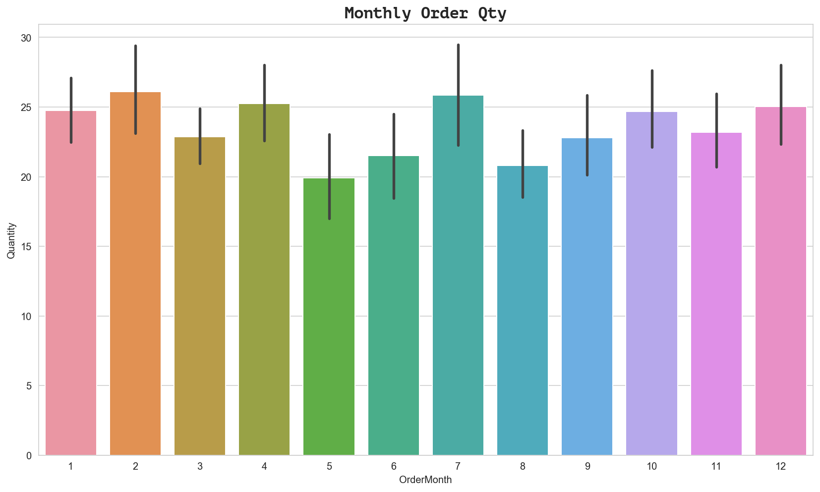
# Check if sample sizes allow us to ignore assumptions;
# visualize sample size comparisons for two groups (normality check)
fig = plt.figure(figsize=(14,8))
ax = fig.gca()
ax = sns.barplot(x='OrderMonth', y='Quantity', data=df_monthly)
ax.set_title('Monthly Order Qty', fontdict={'family': 'PT Mono', 'size':16})

Text(0.5, 1.0, 'Monthly Order Qty')

sns.set_style("whitegrid")
%config InlineBackend.figure_format='retina'
%matplotlib inline


# Check if sample sizes allow us to ignore assumptions;
# visualize sample size comparisons for two groups (normality check)
fig = plt.figure(figsize=(14,8))
ax = fig.gca()
ax = sns.barplot(x='OrderMonth', y='Quantity', data=df_monthly)
ax.set_title('Monthly Order Qty', fontdict={'family': 'PT Mono', 'size':16})

Text(0.5, 1.0, 'Monthly Order Qty')

# Anova Test - Season + Quantity ()

import statsmodels.api as sm
from statsmodels.formula.api import ols
model = ols("Quantity~C(OrderMonth)+Quantity:C(OrderMonth)", data=df_monthly).fit()
anova_table = sm.stats.anova_lm(model, typ=2)
# reformat scientific notation of results for easier interpretation
anova_table.style.format("{:.5f}", subset=['PR(>F)'])

	sum_sq	df	F	PR(>F)
C(OrderMonth)	7395.98	11	2.94204e+29	0.00000
Quantity:C(OrderMonth)	772004	12	2.81504e+31	0.00000
Residual	4.87009e-24	2131	nan	nan

Normality

Statistical

# split orders into two groups (series): discount and fullprice order quantity
Jan = df_monthly.groupby('OrderMonth').get_group(1)['Quantity']

# run tukey test for OQD (Order Quantity Discount) 
data = df_monthly['Quantity'].values
labels = df_monthly['OrderMonth'].values

import statsmodels.api as sms
model = sms.stats.multicomp.pairwise_tukeyhsd(data,labels)

# save OQD tukey test model results into dataframe (OQD: order quantity discount)
tukey_OQD = pd.DataFrame(data=model._results_table[1:], columns=model._results_table[0])
tukey_OQD

	group1	group2	meandiff	p-adj	lower	upper	reject
0	1	2	1.3492	0.9	-4.6052	7.3037	False
1	1	3	-1.8729	0.9	-7.4759	3.73	False
2	1	4	0.5014	0.9	-5.0704	6.0733	False
3	1	5	-4.852	0.358	-11.2668	1.5627	False
4	1	6	-3.2421	0.9	-11.428	4.9438	False
...	...	...	...	...	...	...	...
61	9	11	0.3585	0.9	-6.73	7.4471	False
62	9	12	2.2267	0.9	-4.4923	8.9457	False
63	10	11	-1.5082	0.9	-8.3215	5.3051	False
64	10	12	0.3599	0.9	-6.068	6.7878	False
65	11	12	1.8682	0.9	-4.8142	8.5505	False

66 rows × 7 columns

Results

At a significance level of alpha = 0.05, we reject the null hypothesis which states there is no relationship between time of year (season) and sales revenue or volume of units sold.

Conclusion + Strategic Recommendations

Conclusion & Strategic Recommendations
1. 5% is the minimum discount level needed to produce maximum results.
  - C: Offering discount levels < or > 5% either: a) has no effect on sales revenue and is therefore pointless b) increases loss in revenue despite higher order quantities that could have otherwise been achieved at only 5% discount (thereby maximizing revenue capture/minimizing loss).
  - R: Stop offering any discount other than 5%.
2. Continue to offer discounts in countries where they are effective in producing significantly higher order quantities. Stop offering discounts to countries where there is no effect on order quantities in order to minimize lost revenue.
3. Focus sales and marketing efforts in regions that produce highest revenue; consider
Future Work
- A. Gather and analyze critical missing data on customer types; investigate possible relationships between customer types and product categories (i.e. do certain customer types purchase certain
- C. Investigate possible relationship between regional revenues and shipping cost (i.e. is there a relationship between source (distributor) and destination (shipcountry) that might explain lower revenues in regions that are farther away in physical/geographic distance.

Future Work

Questions to explore in future analyses might include:

Build a product recommendation tool
Create discounts or free shipping offers to increase sales volumes past a certain threshold.
- Shipping Costs and Order Quantities/Sales Revenue Does shipping cost (freight) have a statistically significant effect on quantity? If so, at what level(s) of shipping cost?
Customer Type and Product Category

Is there a relationship between type of customer and certain product categories? If so, we can run more highly targeted sales and marketing programs for increasing sales of certain products to certain market segments.

metricks

What were the top 3 selling products overall?
Top 3 selling products by country?
Top 3 selling products by region?
How did we do in sales for each product category?
Can we group customers into customer types (fill the empty database) and build a product recommendation tool?

# Extract revenue per product category
cur.execute("""SELECT o.OrderId, o.CustomerId, od.ProductId, od.Quantity, od.UnitPrice, 
                od.Quantity*od.UnitPrice*(1-Discount) as Revenue, p.CategoryId, c.CategoryName
                FROM 'Order' o
                JOIN OrderDetail od 
                ON o.OrderId = od.OrderId
                JOIN Product p 
                ON od.ProductId = p.Id
                JOIN Category c
                ON p.CategoryId = c.Id
                ;""")
df = pd.DataFrame(cur.fetchall())
df.columns = [i[0] for i in cur.description]
print(len(df))
df.head(8)

	OrderId	CustomerId	ProductId	Quantity	UnitPrice	Revenue	CategoryId	CategoryName
0	10248	VINET	11	12	14.0	168.0	4	Dairy Products
1	10248	VINET	42	10	9.8	98.0	5	Grains/Cereals
2	10248	VINET	72	5	34.8	174.0	4	Dairy Products
3	10249	TOMSP	14	9	18.6	167.4	7	Produce
4	10249	TOMSP	51	40	42.4	1696.0	7	Produce
5	10250	HANAR	41	10	7.7	77.0	8	Seafood
6	10250	HANAR	51	35	42.4	1261.4	7	Produce
7	10250	HANAR	65	15	16.8	214.2	2	Condiments

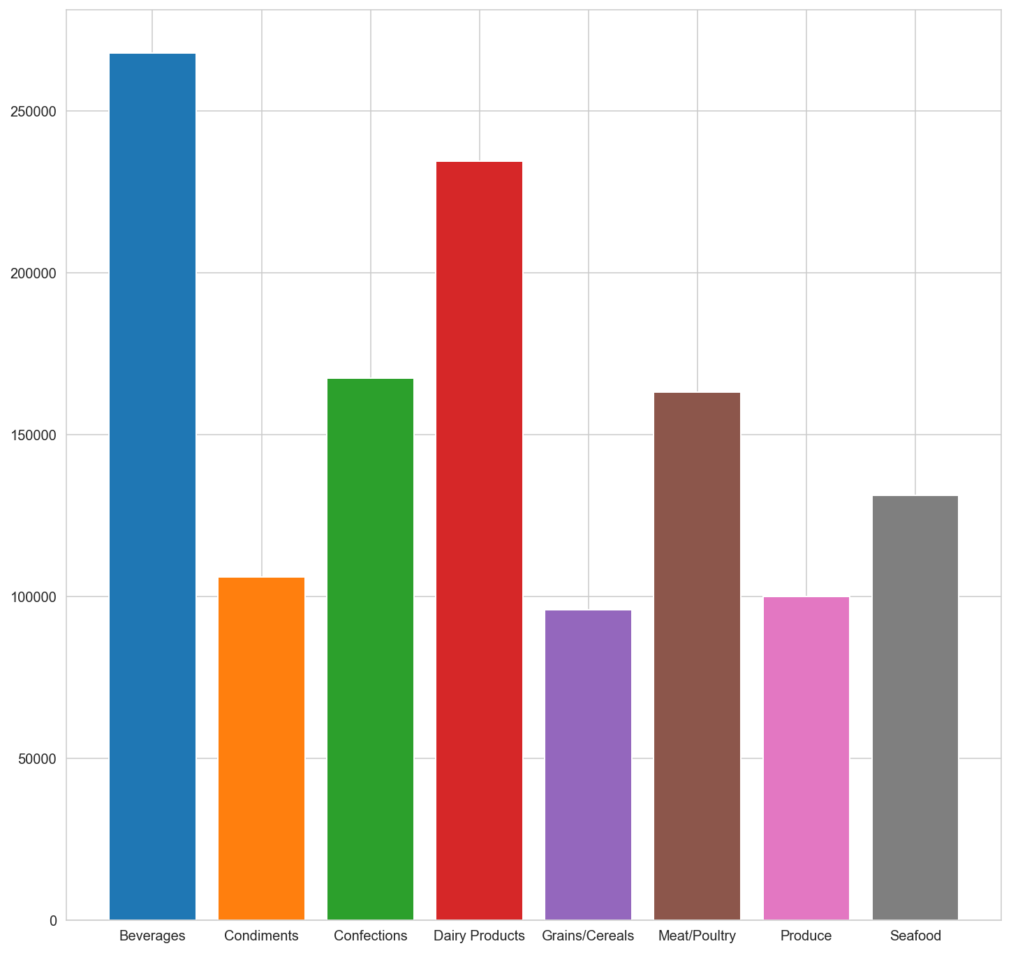
# Group data by Category and get sum total revenue for each
df_category = df.groupby(['CategoryName'])['Revenue'].sum().reset_index()
df_category

	CategoryName	Revenue
0	Beverages	267868.1800
1	Condiments	106047.0850
2	Confections	167357.2250
3	Dairy Products	234507.2850
4	Grains/Cereals	95744.5875
5	Meat/Poultry	163022.3595
6	Produce	99984.5800
7	Seafood	131261.7375

df.CategoryId.value_counts()

  404
  366
  334
  330
  216
  196
  173
  136
Name: CategoryId, dtype: int64

# Explore sample sizes before testing
categories = df.groupby('CategoryName').groups
categories.keys()

dict_keys(['Beverages', 'Condiments', 'Confections', 'Dairy Products', 'Grains/Cereals', 'Meat/Poultry', 'Produce', 'Seafood'])

df_category.loc[df_category['CategoryName'] == 'Beverages']['Revenue'].sum()

267868.17999999993

#create dict of months and order quantity totals
rev_per_cat = {}

for k,v in categories.items():
    rev = df_category.loc[df_category['CategoryName'] == k]['Revenue'].sum()
    rev_per_cat[k] = rev

rev_per_cat

{'Beverages': 267868.17999999993,
 'Condiments': 106047.08500000002,
 'Confections': 167357.22499999995,
 'Dairy Products': 234507.285,
 'Grains/Cereals': 95744.58750000001,
 'Meat/Poultry': 163022.3595,
 'Produce': 99984.57999999999,
 'Seafood': 131261.73750000002}

# plot order quantity totals by month
fig = plt.figure(figsize=(12,12))
for k,v in rev_per_cat.items():
    plt.bar(x=k, height=v)

# What were the top 3 selling product categories in each region or country?
# What were the lowest 3 selling product categories in each region or country?

                       
           /\    _       _                           _                      *  
/\_/\_____/  \__| |_____| |_________________________| |___________________*___
[===]    / /\ \ | |  _  |  _  | _  \/ __/ -__|  \| \_  _/ _  \ \_/ | * _/| | |
 \./    /_/  \_\|_|  ___|_| |_|__/\_\ \ \____|_|\__| \__/__/\_\___/|_|\_\|_|_|
                  | /             |___/        
                  |/   